1 Introduction

This document briefly explains the steps to install and run WRF application on a Virtual Machine deployed in Azure Cloud Platform and presents the performance results.

This recipe document covers the following topics: -

• Deploy & connect a required virtual machine on Azure platform.
• Download & Install Application on virtual machine.
• Performance results of current application on azure virtual machine
• Azure cost
• Summary

2 Deploy Virtual Machine on Azure Cloud Platform

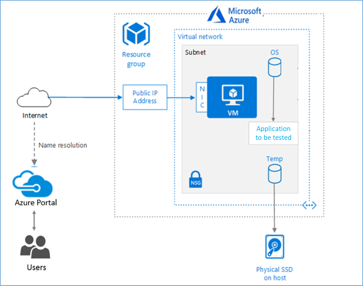
2.1 Azure Cloud Architecture for Application

The below Architecture explains the virtual machine running on an Azure Platform

2.2 Azure Virtual Machine (VM)

A VM is a virtualized instance of a computer that can perform almost all the same functions as a computer, including running applications and operating systems.

An Azure VM gives the flexibility of virtualization without having to buy and maintain the physical hardware that runs it. However, the user still needs to maintain the VM by performing tasks, such as configuring, patching, and installing the software that runs on it.

Things to be considered before deploying a VM:

1. The names of the application resources
2. The location where the resources are stored
3. The size of the VM
4. The operating system that the VM runs
5. The configuration of the VM
6. The related resources that the VM needs

There are different sizes and options available for the Azure virtual machines and user can use to run apps and workloads. Depending on the workload user must choose the appropriate VM size. For complete list check this https://docs.microsoft.com/en-us/azure/virtual-machines/sizes/.

To test the performance of WRF on Azure Platform, below HBv3-series virtual machine is deployed:

The current virtual machine HBv3-series VMs are optimized for HPC applications such as fluid dynamics, explicit and implicit finite element analysis, weather modelling, seismic processing, reservoir simulation, and RTL simulation. HBv3 VMs feature up to 120 AMD EPYC™ 7003-series (Milan) CPU cores, 448 GB of RAM, and no hyperthreading. HBv3-series VMs also provide 350 GB/sec of memory bandwidth; up to 32 MB of L3 cache per core, up to 7 GB/s of block device SSD performance, and clock frequencies up to 3.675 GHz.

2.3 Creation of Virtual Machine

Sign into Azure

Sign into the Azure portal by using https://portal.azure.com/

Free Trial subscriptionsaren't eligible for limit or quota increases.

After the successful sign in or sign up, one has to upgrade the Azure subscription to Pay-As-You-Go to deploy a Virtual machine. For deployment, the user must have regional vCPU quota which can be obtained by raising a request.

The step-by-step procedure to increase the vCPU quota is given in below link:

https://docs.microsoft.com/en-us/azure/azure-portal/supportability/per-vm-quota-requests

The step-by-step procedure to deploy Virtual machine is given below:

1. Type virtual machines in the marketplace search.
2. Under Services, select Virtual machines.
3. In the Virtual machines page, select Create Then Virtual machine.
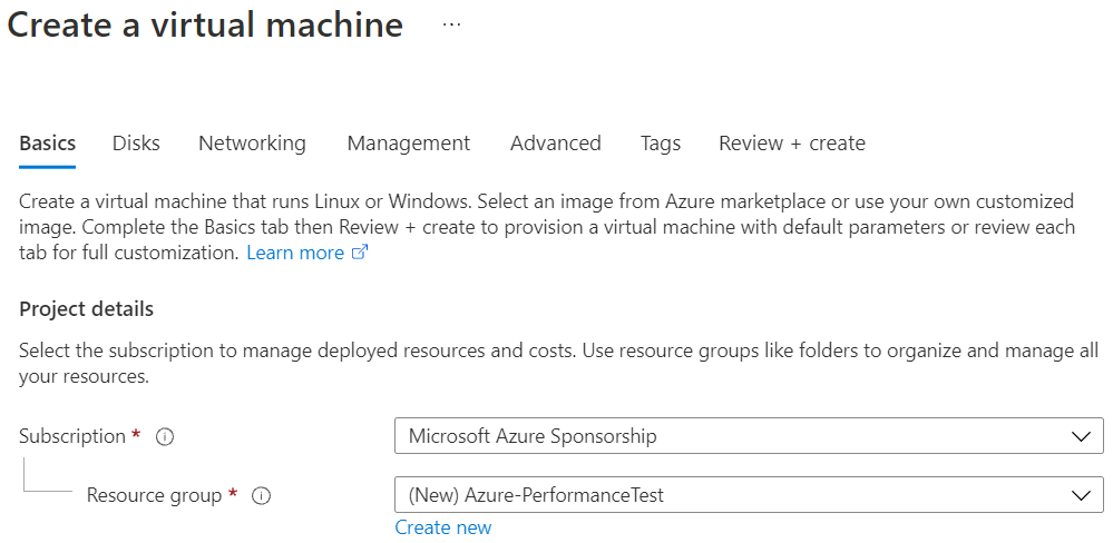
4. In the Basics tab, under Project details, make sure the correct subscription is selected and then choose to Create new resource group. Type Azure-PerformanceTest(user choice) for the name.

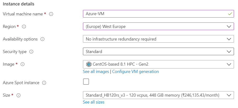
5. Under Instance details, type Azure-VM (user choice) for the Virtual machine name and choose West Europe for Region. Choose CentOS-8.1 HPC-Gen2 for the Image and Standard_HB120rs_v3 for the Size (user choice). Leave the other defaults.

Note:

• Region must be decided based on where the Virtual machine is going to be deployed. To avoid the network latency, the region should be near to the location where the VM is to be deployed.
• Image selection is of user choice based on the application user can choose the image (Windows 10, Linux based OS and Windows Server)

6. Under Administrator account, provide a username, such as Azureuser and a password. The password must be at least 12 characters long and meet the defined complexity requirements.

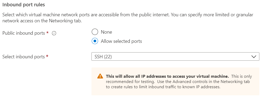
7. Under Inbound port rules, choose Allow selected ports and then select SSH (22) from the drop-down.

8. Leave the remaining defaults and then select the Review + create button at the bottom of the page.
9. After validation runs, select the Create button at the bottom of the page.

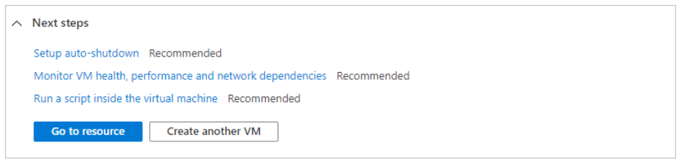
10. After deployment is complete, select Go to resource.

2.4 Connect to virtual machine

Create a SSH connection to the virtual machine.

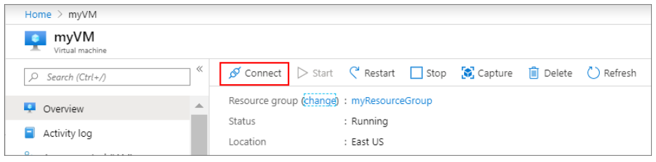
1. On the overview page of a virtual machine, select the Connect button then select SSH and copy the public IP address.

2. Open any SSH client tool of user choice, in this case PUTTY is used.
3. Enter the IP address and port as 22 and click Open

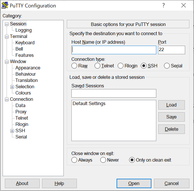
4. Enter username in Login as, enter the password, and click Enter.
5. Now user connected to the VM in Console

3 Install WRF 4.3.1

3.1 Download product

The WRF source code can be obtained from below link:

https://www2.mmm.ucar.edu/wrf/users/download/get_source.html

– Click ‘New Users’, register and download or exiting user can click ‘Returning User’, enter email and download the product.

3.2 Install WRF 4.3.1 on Linux

1. Download source code using steps provided in section 3.1
2. Set up environment for paths and libraries
3. Configure and Compile WRF

For detailed compiling follow the steps provided in below link.

https://www2.mmm.ucar.edu/wrf/OnLineTutorial/compilation_tutorial.php

3.3 Required data for WRF 4.3.1

3.3.1 WRF work flow

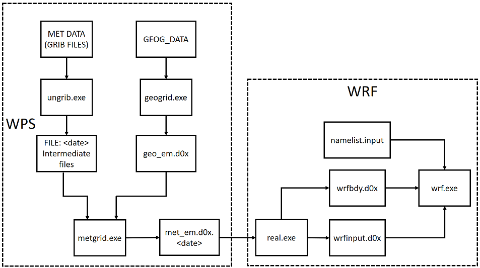
3.3.2 Download static geographic data (for geogrid.exe)

The WRF modelling system is able to create idealized simulations, though most users are interested in the real-data cases. To initiate a real-data case, the domain's physical location on the globe and the static information for that location must be created. This requires a data set that includes such fields as topography and land use categories. These data are available from the WRF download page

http://www2.mmm.ucar.edu/wrf/users/download/get_sources_wps_geog.html

3.3.3 Real time data (for ungrib.exe)

For real-data cases, the WRF model requires up-to-date meteorological information for both an initial condition and also for lateral boundary conditions. This meteorological data is traditionally a Grib file that is provided by a previously run external model or analysis. This data can be downloaded from The National Centres for Environmental Prediction (NCEP) portal in below link.

https://nomads.ncep.noaa.gov

For current simulation below data are downloaded and used to create WPS output files which are the input data files to run the WRF.

https://nomads.ncep.noaa.gov/pub/data/nccf/com/gfs/prod/gfs.20211201/00/atmos/gfs.t00z.pgrb2.0p25.f000

https://nomads.ncep.noaa.gov/pub/data/nccf/com/gfs/prod/gfs.20211201/00/atmos/gfs.t00z.pgrb2.0p25.f003

https://nomads.ncep.noaa.gov/pub/data/nccf/com/gfs/prod/gfs.20211201/00/atmos/gfs.t00z.pgrb2.0p25.f006

https://nomads.ncep.noaa.gov/pub/data/nccf/com/gfs/prod/gfs.20211201/00/atmos/gfs.t00z.pgrb2.0p25.f009

https://nomads.ncep.noaa.gov/pub/data/nccf/com/gfs/prod/gfs.20211201/00/atmos/gfs.t00z.pgrb2.0p25.f012

https://nomads.ncep.noaa.gov/pub/data/nccf/com/gfs/prod/gfs.20211201/00/atmos/gfs.t00z.pgrb2.0p25.f384

3.3.1 WPS output file

One must successfully run WPS, and create met_em. * file for more than one-time period and link or copy WPS output files to the WRF run directory.

Refer to below link to compile & run WPS:

https://www2.mmm.ucar.edu/wrf/OnLineTutorial/compilation_tutorial.php

3.3.2 Defining Model

WRF model (In current case CONUS 2.5 km) is defined by the namelist.input file which will have the model geometric details.

Edit namelist.input file for runtime options (at minimum, one must edit &time control for start, end and integration times, and &domains for grid dimensions)

3.3.3 Configuring options

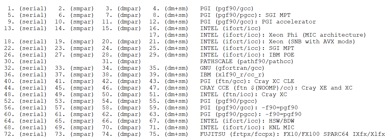
For current performance simulation configuring option 16 (dm+sm) – INTEL (ifort/icc) is selected.

4 Performance Results for WRF 4.3.1

4.1 Overview

The Weather Research and Forecasting (WRF 4.3.1) Model is a next-generation mesoscale numerical weather prediction system designed for both atmospheric research and operational forecasting applications. It features two dynamical cores, a data assimilation system, and a software architecture supporting parallel computation and system extensibility. The model serves a wide range of meteorological applications across scales from tens of meters to thousands of kilometres. The weather research and forecasting (WRF) model is popular in high performance computing (HPC) code used by the weather and climate community. WRF v4 typically performs well on traditional HPC architectures that support high floating-point processing, high memory bandwidth, and a low-latency network

4.2 Model Details

4.3 Azure Platform

When it comes to performance parameters, wall clock time (time taken to complete the simulation) is one parameter, which needs to be analysed. To carry out these simulations on WRF software, right hardware is required. Microsoft partnered with AMD provides the required and suitable Infrastructure and hardware on Azure cloud platform. Microsoft Azure provides the latest and fastest compute capabilities for CPU intensive workloads.

4.4 Performance Results

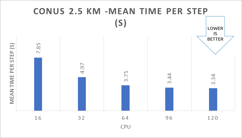
Simulation is carried out to see the performance of chosen Azure VM and the optimised CPU core configuration on single node. Refer chapter 2.2 for the VM specifications.

Thread configuration is an essential parameter to consider when analysing performance since it enhances performance. The thread settings shown below are the best chance for improving hardware performance.

The results were measured by averaging the WRF computation time of each time step from the “rsl.out.0000” output file.

5 Azure Cost

For the below cost reports, the application installation time is not considered and only simulation time is considered for the cost calculation. The Hourly rates reported are subject to change. For the current rate, please refer the link https://azure.microsoft.com/en-in/pricing/calculator/.

6 Summary

1. WRF is successfully deployed and tested on HB120rs_v3 series VM on Azure Platform.
2. Expected meantime per step is achieved in all CPU cores.
3. However, the scalability might vary depending on the dataset being used and the node count being tested. Ensure that to test the impact of the tile size, process, and threads per process before use.

7 Running WRF on Azure Virtual Machines:

Users can use any one of the following two options for the further details:

1. Contact through Microsoft: Microsoft global black belt team
2. Contact through Capgemini: AzureHPC-Certification@capgemini.com